

Where Can I Download A Cat Gc40k Operator Manual?
Note: this post was originally written in June 2016. It is now very outdated. Please see this guide to fine-tuning for an up-to-appointment alternative, or check out chapter 8 of my book "Deep Learning with Python (2d edition)".
In this tutorial, we will present a few simple yet effective methods that you can use to build a powerful image classifier, using only very few training examples --just a few hundred or 1000 pictures from each grade yous want to be able to recognize.
We volition go over the post-obit options:
- training a minor network from scratch (as a baseline)
- using the bottleneck features of a pre-trained network
- fine-tuning the acme layers of a pre-trained network
This will atomic number 82 u.s.a. to comprehend the following Keras features:
-
fit_generatorfor training Keras a model using Python data generators -
ImageDataGeneratorfor real-time data augmentation - layer freezing and model fine-tuning
- ...and more.
Our setup: merely 2000 training examples (1000 per class)
We will start from the post-obit setup:
- a car with Keras, SciPy, PIL installed. If you have a NVIDIA GPU that you can use (and cuDNN installed), that's smashing, but since we are working with few images that isn't strictly necessary.
- a training data directory and validation data directory containing one subdirectory per image class, filled with .png or .jpg images:
data/ train/ dogs/ dog001.jpg dog002.jpg ... cats/ cat001.jpg cat002.jpg ... validation/ dogs/ dog001.jpg dog002.jpg ... cats/ cat001.jpg cat002.jpg ... To acquire a few hundreds or thousands of grooming images belonging to the classes you are interested in, 1 possibility would be to apply the Flickr API to download pictures matching a given tag, nether a friendly license.
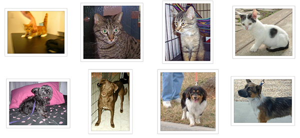
In our examples we will utilise two sets of pictures, which we got from Kaggle: 1000 cats and 1000 dogs (although the original dataset had 12,500 cats and 12,500 dogs, we just took the beginning 1000 images for each form). We also use 400 additional samples from each course every bit validation data, to evaluate our models.
That is very few examples to larn from, for a classification problem that is far from elementary. And so this is a challenging machine learning problem, but it is also a realistic one: in a lot of real-world use cases, fifty-fifty small-calibration information drove tin can be extremely expensive or sometimes near-impossible (e.g. in medical imaging). Being able to brand the most out of very little data is a fundamental skill of a competent data scientist.
How difficult is this problem? When Kaggle started the cats vs. dogs competition (with 25,000 preparation images in full), a chip over two years ago, it came with the following argument:
"In an informal poll conducted many years ago, computer vision experts posited that a classifier with better than 60% accuracy would be difficult without a major advance in the country of the art. For reference, a 60% classifier improves the guessing probability of a 12-image HIP from 1/4096 to 1/459. The current literature suggests machine classifiers tin can score higher up 80% accurateness on this chore [ref]."
In the resulting competition, acme entrants were able to score over 98% accuracy past using modern deep learning techniques. In our instance, because nosotros restrict ourselves to only eight% of the dataset, the problem is much harder.
On the relevance of deep learning for small-data problems
A bulletin that I hear frequently is that "deep learning is only relevant when yous have a huge corporeality of information". While not entirely incorrect, this is somewhat misleading. Certainly, deep learning requires the ability to learn features automatically from the data, which is generally only possible when lots of training data is available --especially for problems where the input samples are very high-dimensional, like images. However, convolutional neural networks --a pillar algorithm of deep learning-- are by design one of the best models bachelor for almost "perceptual" bug (such as image nomenclature), even with very little data to learn from. Training a convnet from scratch on a small image dataset volition still yield reasonable results, without the need for whatever custom feature applied science. Convnets are just manifestly adept. They are the correct tool for the job.
But what's more, deep learning models are by nature highly repurposable: yous can take, say, an prototype nomenclature or spoken language-to-text model trained on a large-scale dataset then reuse information technology on a significantly different trouble with only minor changes, as we volition encounter in this mail service. Specifically in the case of calculator vision, many pre-trained models (usually trained on the ImageNet dataset) are now publicly available for download and can exist used to bootstrap powerful vision models out of very little data.
Data pre-processing and data augmentation
In club to make the virtually of our few grooming examples, we will "broaden" them via a number of random transformations, so that our model would never come across twice the verbal aforementioned picture. This helps prevent overfitting and helps the model generalize ameliorate.
In Keras this tin can be done via the keras.preprocessing.image.ImageDataGenerator class. This class allows y'all to:
- configure random transformations and normalization operations to be washed on your prototype data during training
- instantiate generators of augmented image batches (and their labels) via
.period(data, labels)or.flow_from_directory(directory). These generators can then be used with the Keras model methods that take data generators as inputs,fit_generator,evaluate_generatorandpredict_generator.
Let'due south await at an example correct away:
from keras.preprocessing.image import ImageDataGenerator datagen = ImageDataGenerator ( rotation_range = 40 , width_shift_range = 0.2 , height_shift_range = 0.2 , rescale = 1. / 255 , shear_range = 0.2 , zoom_range = 0.ii , horizontal_flip = True , fill_mode = 'nearest' ) These are just a few of the options available (for more, run across the documentation). Let's quickly become over what we just wrote:
-
rotation_rangeis a value in degrees (0-180), a range inside which to randomly rotate pictures -
width_shiftandheight_shiftare ranges (every bit a fraction of total width or pinnacle) within which to randomly interpret pictures vertically or horizontally -
rescaleis a value past which we will multiply the information before any other processing. Our original images consist in RGB coefficients in the 0-255, but such values would exist also high for our models to procedure (given a typical learning rate), then we target values between 0 and 1 instead by scaling with a one/255. cistron. -
shear_rangeis for randomly applying shearing transformations -
zoom_rangeis for randomly zooming within pictures -
horizontal_flipis for randomly flipping half of the images horizontally --relevant when there are no assumptions of horizontal assymetry (e.g. existent-world pictures). -
fill_modeis the strategy used for filling in newly created pixels, which tin appear after a rotation or a width/height shift.
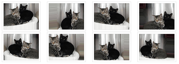
Now let's start generating some pictures using this tool and salvage them to a temporary directory, so we can become a feel for what our augmentation strategy is doing --we disable rescaling in this case to proceed the images displayable:
from keras.preprocessing.paradigm import ImageDataGenerator , array_to_img , img_to_array , load_img datagen = ImageDataGenerator ( rotation_range = 40 , width_shift_range = 0.two , height_shift_range = 0.2 , shear_range = 0.2 , zoom_range = 0.2 , horizontal_flip = True , fill_mode = 'nearest' ) img = load_img ( 'data/railroad train/cats/true cat.0.jpg' ) # this is a PIL image 10 = img_to_array ( img ) # this is a Numpy array with shape (3, 150, 150) x = x . reshape (( ane ,) + ten . shape ) # this is a Numpy array with shape (1, three, 150, 150) # the .menstruation() control below generates batches of randomly transformed images # and saves the results to the `preview/` directory i = 0 for batch in datagen . flow ( x , batch_size = 1 , save_to_dir = 'preview' , save_prefix = 'cat' , save_format = 'jpeg' ): i += 1 if i > twenty : break # otherwise the generator would loop indefinitely Here'southward what we get --this is what our information augmentation strategy looks like.
Training a small convnet from scratch: 80% accuracy in 40 lines of lawmaking
The right tool for an epitome classification task is a convnet, so allow's try to railroad train one on our data, as an initial baseline. Since we simply take few examples, our number one business organization should be overfitting. Overfitting happens when a model exposed to too few examples learns patterns that do non generalize to new data, i.e. when the model starts using irrelevant features for making predictions. For instance, if you, as a human, only meet three images of people who are lumberjacks, and three, images of people who are sailors, and amongst them only 1 lumberjack wears a cap, yous might starting time thinking that wearing a cap is a sign of beingness a lumberjack as opposed to a sailor. Yous would and then brand a pretty lousy lumberjack/sailor classifier.
Data augmentation is one way to fight overfitting, merely it isn't enough since our augmented samples are still highly correlated. Your main focus for fighting overfitting should exist the entropic capacity of your model --how much information your model is allowed to store. A model that can store a lot of information has the potential to exist more accurate past leveraging more features, but information technology is also more than at risk to beginning storing irrelevant features. Meanwhile, a model that can only store a few features will have to focus on the nearly pregnant features found in the data, and these are more than likely to be truly relevant and to generalize better.
There are different ways to modulate entropic chapters. The primary ane is the choice of the number of parameters in your model, i.e. the number of layers and the size of each layer. Another way is the use of weight regularization, such as L1 or L2 regularization, which consists in forcing model weights to taker smaller values.
In our case we volition use a very small convnet with few layers and few filters per layer, alongside information augmentation and dropout. Dropout also helps reduce overfitting, by preventing a layer from seeing twice the exact same blueprint, thus acting in a way analoguous to data augmentation (you could say that both dropout and data augmentation tend to disrupt random correlations occuring in your information).
The code snippet beneath is our first model, a elementary stack of 3 convolution layers with a ReLU activation and followed by max-pooling layers. This is very similar to the architectures that Yann LeCun advocated in the 1990s for image classification (with the exception of ReLU).
The total code for this experiment can be found hither.
from keras.models import Sequential from keras.layers import Conv2D , MaxPooling2D from keras.layers import Activation , Dropout , Flatten , Dumbo model = Sequential () model . add ( Conv2D ( 32 , ( 3 , iii ), input_shape = ( 3 , 150 , 150 ))) model . add ( Activation ( 'relu' )) model . add ( MaxPooling2D ( pool_size = ( ii , 2 ))) model . add ( Conv2D ( 32 , ( 3 , three ))) model . add ( Activation ( 'relu' )) model . add ( MaxPooling2D ( pool_size = ( 2 , ii ))) model . add together ( Conv2D ( 64 , ( 3 , three ))) model . add together ( Activation ( 'relu' )) model . add ( MaxPooling2D ( pool_size = ( 2 , two ))) # the model so far outputs 3D feature maps (pinnacle, width, features) On top of information technology we stick two fully-connected layers. We end the model with a single unit and a sigmoid activation, which is perfect for a binary nomenclature. To become with it we will likewise use the binary_crossentropy loss to train our model.
model . add ( Flatten ()) # this converts our 3D feature maps to 1D feature vectors model . add ( Dense ( 64 )) model . add ( Activation ( 'relu' )) model . add ( Dropout ( 0.5 )) model . add together ( Dense ( 1 )) model . add ( Activation ( 'sigmoid' )) model . compile ( loss = 'binary_crossentropy' , optimizer = 'rmsprop' , metrics = [ 'accuracy' ]) Allow's gear up our data. We will employ .flow_from_directory() to generate batches of image information (and their labels) directly from our jpgs in their corresponding folders.
batch_size = xvi # this is the augmentation configuration we will use for preparation train_datagen = ImageDataGenerator ( rescale = 1. / 255 , shear_range = 0.2 , zoom_range = 0.2 , horizontal_flip = True ) # this is the augmentation configuration we will use for testing: # only rescaling test_datagen = ImageDataGenerator ( rescale = 1. / 255 ) # this is a generator that will read pictures found in # subfolers of 'information/train', and indefinitely generate # batches of augmented image information train_generator = train_datagen . flow_from_directory ( 'data/train' , # this is the target directory target_size = ( 150 , 150 ), # all images will exist resized to 150x150 batch_size = batch_size , class_mode = 'binary' ) # since we use binary_crossentropy loss, we demand binary labels # this is a similar generator, for validation data validation_generator = test_datagen . flow_from_directory ( 'information/validation' , target_size = ( 150 , 150 ), batch_size = batch_size , class_mode = 'binary' ) Nosotros can at present apply these generators to train our model. Each epoch takes xx-30s on GPU and 300-400s on CPU. Then it's definitely viable to run this model on CPU if you aren't in a hurry.
model . fit_generator ( train_generator , steps_per_epoch = 2000 // batch_size , epochs = fifty , validation_data = validation_generator , validation_steps = 800 // batch_size ) model . save_weights ( 'first_try.h5' ) # ever save your weights after preparation or during preparation This approach gets us to a validation accuracy of 0.79-0.81 afterwards 50 epochs (a number that was picked arbitrarily --because the model is small and uses ambitious dropout, it does non seem to be overfitting too much by that bespeak). So at the time the Kaggle competition was launched, we would be already exist "state of the art" --with viii% of the data, and no try to optimize our architecture or hyperparameters. In fact, in the Kaggle competition, this model would have scored in the top 100 (out of 215 entrants). I guess that at to the lowest degree 115 entrants weren't using deep learning ;)
Note that the variance of the validation accurateness is fairly high, both considering accuracy is a high-variance metric and because we only apply 800 validation samples. A proficient validation strategy in such cases would be to practice k-fold cross-validation, but this would require training 1000 models for every evaluation round.
Using the clogging features of a pre-trained network: 90% accuracy in a minute
A more refined approach would be to leverage a network pre-trained on a large dataset. Such a network would accept already learned features that are useful for most computer vision problems, and leveraging such features would allow the states to reach a better accuracy than whatsoever method that would only rely on the available data.
We will apply the VGG16 architecture, pre-trained on the ImageNet dataset --a model previously featured on this blog. Because the ImageNet dataset contains several "true cat" classes (farsi cat, siamese cat...) and many "canis familiaris" classes amid its full of thousand classes, this model will already accept learned features that are relevant to our classification problem. In fact, it is possible that merely recording the softmax predictions of the model over our data rather than the clogging features would be enough to solve our dogs vs. cats classification trouble extremely well. However, the method we nowadays here is more likely to generalize well to a broader range of problems, including issues featuring classes absent-minded from ImageNet.
Here's what the VGG16 architecture looks like:
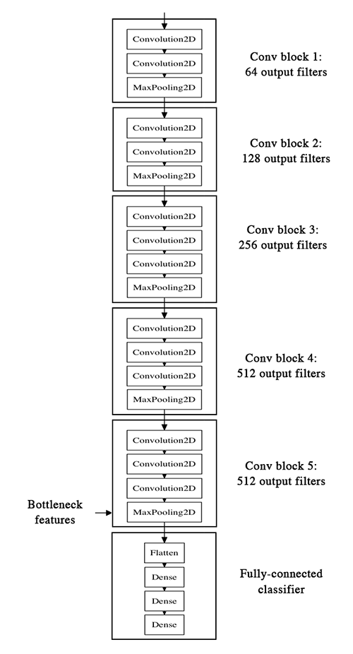
Our strategy will be every bit follow: we volition merely instantiate the convolutional part of the model, everything upwardly to the fully-connected layers. We will then run this model on our training and validation data one time, recording the output (the "bottleneck features" from th VGG16 model: the final activation maps earlier the fully-connected layers) in two numpy arrays. Then we will train a small fully-connected model on top of the stored features.
The reason why nosotros are storing the features offline rather than adding our fully-connected model directly on summit of a frozen convolutional base of operations and running the whole thing, is computational effiency. Running VGG16 is expensive, particularly if you lot're working on CPU, and we want to but do it in one case. Note that this prevents us from using data augmentation.
You can notice the full code for this experiment hither. Y'all can become the weights file from Github. We won't review how the model is built and loaded --this is covered in multiple Keras examples already. But permit's accept a look at how we record the bottleneck features using epitome data generators:
batch_size = 16 generator = datagen . flow_from_directory ( 'data/train' , target_size = ( 150 , 150 ), batch_size = batch_size , class_mode = None , # this means our generator volition only yield batches of data, no labels shuffle = Faux ) # our information will be in order, and so all first thousand images will exist cats, then 1000 dogs # the predict_generator method returns the output of a model, given # a generator that yields batches of numpy data bottleneck_features_train = model . predict_generator ( generator , 2000 ) # save the output every bit a Numpy assortment np . save ( open ( 'bottleneck_features_train.npy' , 'west' ), bottleneck_features_train ) generator = datagen . flow_from_directory ( 'information/validation' , target_size = ( 150 , 150 ), batch_size = batch_size , class_mode = None , shuffle = False ) bottleneck_features_validation = model . predict_generator ( generator , 800 ) np . salvage ( open up ( 'bottleneck_features_validation.npy' , 'w' ), bottleneck_features_validation ) We can then load our saved data and railroad train a pocket-size fully-continued model:
train_data = np . load ( open ( 'bottleneck_features_train.npy' )) # the features were saved in social club, so recreating the labels is piece of cake train_labels = np . array ([ 0 ] * g + [ 1 ] * thou ) validation_data = np . load ( open ( 'bottleneck_features_validation.npy' )) validation_labels = np . array ([ 0 ] * 400 + [ 1 ] * 400 ) model = Sequential () model . add together ( Flatten ( input_shape = train_data . shape [ 1 :])) model . add ( Dumbo ( 256 , activation = 'relu' )) model . add together ( Dropout ( 0.v )) model . add ( Dense ( i , activation = 'sigmoid' )) model . compile ( optimizer = 'rmsprop' , loss = 'binary_crossentropy' , metrics = [ 'accurateness' ]) model . fit ( train_data , train_labels , epochs = 50 , batch_size = batch_size , validation_data = ( validation_data , validation_labels )) model . save_weights ( 'bottleneck_fc_model.h5' ) Thanks to its small-scale size, this model trains very quickly even on CPU (1s per epoch):
Train on 2000 samples, validate on 800 samples Epoch 1/l 2000/2000 [==============================] - 1s - loss: 0.8932 - acc: 0.7345 - val_loss: 0.2664 - val_acc: 0.8862 Epoch 2/50 2000/2000 [==============================] - 1s - loss: 0.3556 - acc: 0.8460 - val_loss: 0.4704 - val_acc: 0.7725 ... Epoch 47/50 2000/2000 [==============================] - 1s - loss: 0.0063 - acc: 0.9990 - val_loss: 0.8230 - val_acc: 0.9125 Epoch 48/50 2000/2000 [==============================] - 1s - loss: 0.0144 - acc: 0.9960 - val_loss: 0.8204 - val_acc: 0.9075 Epoch 49/50 2000/2000 [==============================] - 1s - loss: 0.0102 - acc: 0.9960 - val_loss: 0.8334 - val_acc: 0.9038 Epoch 50/50 2000/2000 [==============================] - 1s - loss: 0.0040 - acc: 0.9985 - val_loss: 0.8556 - val_acc: 0.9075 We reach a validation accurateness of 0.ninety-0.91: not bad at all. This is definitely partly due to the fact that the base model was trained on a dataset that already featured dogs and cats (among hundreds of other classes).
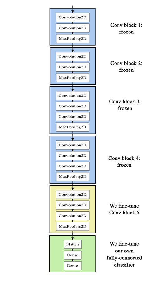
Fine-tuning the top layers of a a pre-trained network
To further ameliorate our previous result, we tin try to "fine-tune" the last convolutional block of the VGG16 model aslope the top-level classifier. Fine-tuning consist in starting from a trained network, then re-training it on a new dataset using very small weight updates. In our case, this tin exist done in 3 steps:
- instantiate the convolutional base of VGG16 and load its weights
- add together our previously defined fully-connected model on superlative, and load its weights
- freeze the layers of the VGG16 model up to the last convolutional cake
Note that:
- in order to perform fine-tuning, all layers should kickoff with properly trained weights: for instance you should not slap a randomly initialized fully-connected network on acme of a pre-trained convolutional base. This is because the big gradient updates triggered by the randomly initialized weights would wreck the learned weights in the convolutional base. In our case this is why we commencement train the height-level classifier, and only then beginning fine-tuning convolutional weights alongside it.
- we choose to merely fine-tune the concluding convolutional block rather than the unabridged network in order to foreclose overfitting, since the entire network would have a very big entropic capacity and thus a strong trend to overfit. The features learned past depression-level convolutional blocks are more than general, less abstract than those found higher-up, so it is sensible to continue the first few blocks fixed (more than general features) and just fine-melody the last i (more specialized features).
- fine-tuning should be done with a very tedious learning rate, and typically with the SGD optimizer rather than an adaptative learning rate optimizer such every bit RMSProp. This is to make sure that the magnitude of the updates stays very small, so as not to wreck the previously learned features.
Y'all tin discover the full code for this experiment here.
After instantiating the VGG base and loading its weights, nosotros add our previously trained fully-connected classifier on pinnacle:
# build a classifier model to put on top of the convolutional model top_model = Sequential () top_model . add together ( Flatten ( input_shape = model . output_shape [ one :])) top_model . add ( Dense ( 256 , activation = 'relu' )) top_model . add ( Dropout ( 0.v )) top_model . add ( Dense ( 1 , activation = 'sigmoid' )) # note that information technology is necessary to start with a fully-trained # classifier, including the top classifier, # in guild to successfully practice fine-tuning top_model . load_weights ( top_model_weights_path ) # add the model on top of the convolutional base of operations model . add ( top_model ) We so proceed to freeze all convolutional layers up to the last convolutional block:
# set the commencement 25 layers (up to the last conv block) # to non-trainable (weights will not be updated) for layer in model . layers [: 25 ]: layer . trainable = False # compile the model with a SGD/momentum optimizer # and a very boring learning rate. model . compile ( loss = 'binary_crossentropy' , optimizer = optimizers . SGD ( lr = 1e-four , momentum = 0.9 ), metrics = [ 'accuracy' ]) Finally, we offset training the whole thing, with a very boring learning rate:
batch_size = 16 # ready information augmentation configuration train_datagen = ImageDataGenerator ( rescale = 1. / 255 , shear_range = 0.two , zoom_range = 0.ii , horizontal_flip = True ) test_datagen = ImageDataGenerator ( rescale = 1. / 255 ) train_generator = train_datagen . flow_from_directory ( train_data_dir , target_size = ( img_height , img_width ), batch_size = batch_size , class_mode = 'binary' ) validation_generator = test_datagen . flow_from_directory ( validation_data_dir , target_size = ( img_height , img_width ), batch_size = batch_size , class_mode = 'binary' ) # fine-tune the model model . fit_generator ( train_generator , steps_per_epoch = nb_train_samples // batch_size , epochs = epochs , validation_data = validation_generator , validation_steps = nb_validation_samples // batch_size ) This approach gets us to a validation accuracy of 0.94 after 50 epochs. Great success!
Here are a few more approaches you tin can try to become to in a higher place 0.95:
- more aggresive information augmentation
- more aggressive dropout
- use of L1 and L2 regularization (also known as "weight disuse")
- fine-tuning ane more convolutional cake (aslope greater regularization)
This mail ends here! To recap, here is where yous tin can find the lawmaking for our three experiments:
- Convnet trained from scratch
- Bottleneck features
- Fine-tuning
If you take whatsoever comment about this post or whatsoever proffer most futurity topics to cover, you tin accomplish out on Twitter.

Source: https://blog.keras.io/building-powerful-image-classification-models-using-very-little-data.html
Posted by: jenningsdever1949.blogspot.com
0 Response to "Where Can I Download A Cat Gc40k Operator Manual?"
Post a Comment